Statistical learning with R part 4: Clustering
[This post is part of the Statistical learning with R series]
If you are here you probably have already unpacked the tgz file containing the demos and read the previous articles (part 1: Overfitting and part 2: Linear regression, and part 3: Classification). If not, please check this page before starting.
Try to run clusteringDemo.R: supposing your current working directory is the one where you unpacked the R files, type
source("clusteringDemo.R",print.eval=TRUE)
The print.eval parameter is needed to show you the output of some commands such as summary in the context of the source command. Also remember that the demo generates some random data and before running it you should edit it and set up your own random seed.
This demo tests different clustering algorithms (K-Means, Hierarchical, and K-Medoids) on the Iris flower dataset.
After you run the full demo, try to answer the following questions:
- What can you say about the WSS vs K plot? Can you spot an elbow? How can you interpret this behaviour, knowing the correct K and having looked at how the dataset looks like?
- What kind of hierarchical clustering is ran by default? Top down or bottom up? Single, complete, or average linkage? Can you modify the method (just look at the parameters of the hclust function) to obtain better results in terms of NMI?
- Try to play with the fuzziness coefficient parameter (m) of Fuzzy C-Means. We know that its value is strictly greater than 1 but with no upper bound. What happens if its value is very close to 1? What happens if it is very big? And what if the value is the default (2)?
- What is the best algorithm in terms of NMI (also take into account the different methods of Hierarchical)? Which one do you consider the best in terms of interpretability of the results?
- Finally, take one sample whose Fuzzy C-Means membership does not clearly put it in one cluster (you can look at the "Memberships" matrix printed after FCM execution, check e.g. sample 51). What makes it so ambiguous? Try to check its features (iris[51,]) and the ones of the cluster centers (i.e. the representative points of each cluster, result$centers), and comment what you found.
Statistical learning with R part 3: Classification
[This post is part of the Statistical learning with R series]
If you are here you probably have already unpacked the tgz file containing the demos and read the previous articles (part 1: Overfitting and part 2: Linear regression). If not, please check this page before starting.
Try to run classificationDemo.R: supposing your current working directory is the one where you unpacked the R files, type
source("classificationDemo.R",print.eval=TRUE)
The print.eval parameter is needed to show you the output of some commands such as summary in the context of the source command. Also remember that the demo generates some random data and before running it you should edit it and set up your own random seed.
This demo shows you two different classification experiments. In the former, you will run your own spam filter on the HP Labs SPAM E-mail Database. In the latter, you will use classification to recognise handwritten digits from the USPS ZIP code dataset (Le Cun et al., 1990). You can find more information on both of the datasets here, in the "Data" section.
After you run the full demo, try to answer the following questions:
- Look at the confusion matrix from logistic regression and interpret it. How many messages have been correctly classified as spam? How many as non-spam? How many false positives you have (e.g. messages classified as spam that were not)? And how many false negatives?
- The spam experiment runs by default with a given training set (provided by the dataset creators for an easier comparison with other methods). Try to change it with a random one (all the code is ready for you to use within the script). Does anything significative change if you do this? What if you change the default size of the set?
- If you think about the spam experiment as a *real* problem, you might not just settle with a solution which gives you the smallest error, but you'd probably want to also minimize the *false positives* (i.e. you do not want to classify regular messages as spam). Play with the threshold to reduce the number of false positives and discuss the results: how does the general error change? How does the amount of spam you cannot recognize anymore increase?
- In the digits classification experiment, what is the digit that is misclassified the most by QDA? Try to display some examples of this misclassified digit (all the code you need is available in the script)
- Compare the results given by the different classification approaches in *both experiments*. What are the best ones? Relying on the methods comparison in your textbook, can you provide hypotheses explaining this behaviour?
Statistical learning with R part 2: Linear regression
[This post is part of the Statistical learning with R series]
So, if you are here you probably have already unpacked the tgz file containing the demos and read the previous article about overfitting. If not, please check this page before starting.
Try to run linearRegressionDemo.R: supposing your current working directory is the one where you unpacked the R files, type
source("linearRegressionDemo.R",print.eval=TRUE)
The print.eval parameter is needed to show you the output of some commands such as summary in the context of the source command. Also remember that the demo generates some random data and before running it you should edit it and set up your own random seed.
This demo performs different linear regressions on the Los Angeles ozone dataset (simple, multivariate, with non-linear extensions, etc.). After you run the full demo, try to answer the following questions:
- The variable selection results we obtain with the regsubsets command are consistent with the first three steps we performed manually. Can you tell which approach we used for variable selection (both in regsubsets and in manual selection)? Would the sets of selected variables be the same if we chose another approach in regsubsets?(NOTE: you can try that! Just type ?regsubsets in R to see which methods are allowed, and change the current one in the code
- Which is the best variable selection method in qualitative terms? Choose e.g. the sets of 4 variables you get with the different methods provided by regsubsets, fit linear models using them, and show which one has the lowest MSE. Can you also explain why that method is better?
- Just by introducing a very simple non-linearity in our model we were able to get a better fit both in the training and in the test sets. Can you do better? Try to modify the code to include other types of non-linearities (in the simplest case, more complex polynomials) and verify whether the model
gets better only in the training set or also in test. - What can you say about the final results, comparing the evaluations of the training and test sets? Do you think there is actually overfitting? Do things change if you choose different values for the training and test sets?
Statistical learning with R part 1: Overfitting
[This post is part of the Statistical learning with R series]
So, if you are here you probably have already unpacked the tgz file containing the demos and done your first experiments trying to run R scripts. If not, please check this page before starting.
Try to run overfittingDemo.R: supposing your current working directory is the one where you unpacked the R files, you can just type
source("overfittingDemo.R",print.eval=TRUE)
(note that each demo generates some random data and before running one you should edit it and set up your own random seed).
In the overfitting demo you will generate different datasets, try to fit more and more flexible functions to the data, and evaluate how good your functions are in terms of how well they fit both a training and a test dataset. After you run the full demo, try to answer the following questions:
- We have seen that increasing the flexibility we tend to overfit the data, i.e. while the training MSE gets smaller, the test MSE increases. Is the opposite also true for our datasets, i.e. is the simplest, less flexible function taken into consideration the one that also provides the smallest test MSE? If not, can you explain why?
- How good are our errors? Throughout the whole demo, we have talked about errors without ever referring to the smallest possible one that we can get, that is the irreducible error. How is it calculated and what is its size in each of the generated datasets?
- The default datasets are quite small, and in some cases (e.g. try with seed=789) the results are not exactly the expected ones. Do results change sensibly if you increase the number of points? Can you tell why? (NOTE: you can do that just by changing the dataset_size variable at the beginning of the script)
Statistical learning with R – Introduction and setup
New year, new PAMI class: as the format changed with respect to previous years, my homeworks/demos are also different, and you will need R to run them. If you have not played with R yet, the notes I have attached to the introductory Lab might be of help.
If you attended the class, you probably know what to do with the next posts. After you have ran each demo, answer the related questions you will find both in the blog post and in the demo itself. Add whatever is necessary (screenshots, code, text, links) to motivate your answers and convince me you actually ran the demos and understood them. Finally send me everything in a pdf file.
To run each demo, just open the R file you will find in each post with the source command in R, for example:
source("/whatever/your/path/is/demofilename.R",print.eval = TRUE)
For your convenience, here is a package containing all of the source and data files you need for your homework (the package will be updated every time a new demo is added). Remember that while you will not be asked to add much new code to the demos, you should at least be able to understand what it does and modify some parameters to produce different results. Now feel free to play with the following demos:
Octave clustering demo part 6: (more) evaluation
[This post is part of the Octave clustering demo series]
This new clustering demo goes deeper into evaluation, showing some techniques to get an idea about the clustering tendency of a dataset, find visual clues about the clusters, and get a hint about the "best" number of clusters. If you have attended the PAMI class this year you probably know what I am talking about. If instead you are new to these demos please (1) check the page linked above and (2) set up your Octave environment (feel free to download the old package and play with the old demos too ;-)). Then download this new package.
If you want to check out the older Octave clustering articles, here they are: part 0 - part 1 - part 2 - part 3 - part 4 - part 5. I strongly suggest you to run at least parts 0-3 before this demo, as they provide you all the basics you need to get the best out of this exercise.
Note that some of the functions available in previous packages are also present in this one. While it is ok to run the previous examples with those functions, make sure you are using the most up-to-date ones for the current experiments, as I debugged and optimized them for this specific demo.
Run the evaluationDemo1 script. This will generate a random dataset and walk you through a sequence of tests to evaluate the clustering tendency and ultimately perform clustering on it. As random clusters might be more or less nasty to cluster, I suggest you to try running the demo few times and see how it behaves in general. Note that part of the code is missing and you will have to provide it for the demo to be complete.
When you feel confident enough with evaluating the random dataset, run the evaluationDemo2 script. This will be a little more interactive, asking you to choose, between three datasets, the one which has the most "interesting" content, and requiring you to write small pieces of code to complete your evaluation.
At the end of your experiment, answer the following questions:
- comment the different executions of evaluationDemo1. How sensitive to "bad" overlapping clusters are SSE elbow and distance matrix plot? Does the presence of overlapping clusters affect the clustering tendency test? How do you think it would be possible (and in this case, would it be meaningful) to distinguish between two completely overlapping clusters?
- comment the different executions of evaluationDemo2. Which is the "interesting" dataset? Why? Is the SSE elbow method useful to automatically detect the number of clusters? Why? What additional information does the distance matrix convey? Is Spectral clustering better than k-Means? Did you happen to find parameters that give better accuracy than the default ones?
If you are a PAMI student, please write your answers in a pdf file, motivating them and providing all the material (images, code, numerical results) needed to support them.
Hints:
- the demo stops at each step waiting for you to press a key. You can disable this feature by setting the "interactive" variable to zero at the beginning of the script;
- the second demo file has some "return" commands purposely left in the code to stop the execution at given points (typically when you need to add some code before proceeding, or to increase the suspance ;-));
- I tested the code on Octave (3.6.4) and MATLAB (2011a) and it runs on both. If you still have problems please let me know ASAP and we will sort them out.
Octave clustering demo part 5: hierarchical clustering
[This post is part of the Octave clustering demo series]
So, if you read this you probably have already unpacked the tgz file containing the demo and read the previous article about k-medoids clustering. If you want to check out the older Octave clustering articles, here they are: part 0 - part 1 - part 2 - part 3.
Run the hierarchicalDemo script (if launched without input parameters, it will open the "crescents.mat" data file by default). The script will plot the dataset, then it will try to perform clustering using first k-means and then an agglomerative hierarchical clustering algorithm. Run the algorithm with all the datasets available (note that you will need to modify the code to make it work with different numbers of clusters).
Questions:
- how does k-means perform on the non-globular datasets (crescents, circles01, and circles02)? What is the reason of this performance? how does hierarchical algorithm perform instead?
- now let us play with the "agglomerative" dataset. Information is missing so you know neither the number of clusters in advance nor the ground truth about points (i.e. which class they belong to). First of all, run the hclust function with different numbers of clusters and plot the results. Are you satisfied with them? What do you think is the reason of this "chaining" phenomenon?
- complete the code in hclust.m so it also calculates complete and average linkage, and run the algorithm again. How do clustering results change? Plot and comment them.
Octave clustering demo part 4: k-Medoids
[This post is part of the Octave clustering demo series]
Here follows the description of the first of two new Octave clustering demos. If you have attended the PAMI class this year you probably know what I am talking about. If instead you are new to these demos please (1) check the page linked above and (2) set up your Octave environment (feel free to download the old package and play with the old demos too ;-)). Then download this new package.
Run the kMedoidsDemo script (if launched without input parameters, it will open the "noisyBlobs01.mat" data file by default). The script will plot the dataset, then it will try to perform clustering using first k-means and then k-medoids. Run the experiment many times (at least 4-5 times) for each of the three noisyBlobs datasets (you can pass the dataset path and name as a parameter to the kMedoidsDemo function).
Questions:
- comment the "worst case" results you get from k-means: what happens and how does noise influence this behavior?
- compare the results you get with k-means with the ones you get with k-medoids: how does k-medoids deal with the presence of noise?
- what would happen if noise points were much farther from the original clusters? Try to get few (1-2) of them and bring them very far from the rest of the data… what are the results you get from k-means and k-medoids?
Hints:
- the demo stops at each step waiting for you to press a key. You can disable this feature by setting the "interactive" variable to zero at the beginning of the script;
- there are two different k-means implementations you can run: feel free to try both just by uncommenting their respective code.
WordPress in a (Virtual)box
Looking for some cool material for a new class at SUPSI DFA, I recently had a chance to experiment with Virtual Appliances. The main idea is the following: to setup most Web applications you need not only the applications themselves, but a whole set of softwares they depend on, (e.g. a web server, a database, a language interpreter), some additional apps to manage your data (e.g. phpMyAdmin to administer your MySQL database), and of course configurations for all of them; a virtual appliance is a self-contained virtual machine where everything, from the OS to every bit of code you need, is already installed and configured so that you won't need to worry about setting up your system, but you will be immediately able to start working with it.
There exist different VA providers, such as Bitnami, Turnkey Linux, and JumpBox. Each one has its own peculiarities: for instance, JumpBox uses proprietary software (as far as I learned from here) and to get VA images you need to pay a subscription; Bitnami does not only provide virtual machines, but also native installers for Windows, Linux, and Mac, and all of these are free; TKL, also free, is oriented to more technical users and should be better if you plan to extend the VA with other services, as (since August 2012) it is based on a standard Debian installation.
Ok, ok, now I guess you are curious about what virtual appliances are actually available. Of course you can find WordPress (e.g. here and here) as in this post's title, but also content management systems such as Drupal and Joomla, wikis as MediaWiki and MoinMoin, torrent servers, Web frameworks such as Django, developers stacks (e.g. *AMP, *APP), and revision control servers. So I guess this post is going to provide you a veeeery limited view on what you can do, but I hope it will at least stimulate some curiosity in you (then probably other posts will follow with new discoveries… ;-)).
My first experiment with these VAs has been with Bitnami's WordPress. There are three ways to install it: using the native installer, with a VM image or directly deploying it in a cloud, e.g. on Windows Azure or AWS. The native installer on Mac is quite straightforward: you install it, provide (relatively) few configuration parameters, and voilà, you are ready to connect to your IP address (port 8080) and use your new WordPress or access your DB via phpmyadmin. All of this without being scared by the presence of all these new softwares in your system: everything is self-contained in one directory and does not interfere with existing software. For instance, I already have a MySQL instance running on my Mac and I just needed to provide a different port to make the two coexist.
This is very convenient if you want to test a new Web application. Its main limitation, however, is that it runs on your own PC, so if you want to make that WordPress website (or in general any Bitnami system you are running) accessible somewhere in the cloud, starting with a virtual appliance is going to make your life much easier.
Running the virtual appliance is also quite simple both with VMWare and with Virtualbox. In the latter case, converting the virtual disk from the VMDK (VMWare) to the VDI (Virtualbox) format is required. Be sure you check the virtual appliances quick start guide here, then perform the following steps.
Step 0: as a pre-requirement, I suppose you already have a recent version of VirtualBox installed. The one I am working with now is 4.2.6. If you don't, get one here.
Step 1: download the latest virtual appliance image file (e.g. for WordPress, get it here) and unzip it (at the time of writing this post, the filename is bitnami-wordpress-3.5-0-ubuntu-12.04.zip). This will create a new directory with the same name of the file (except the ".zip" extension, of course).
Step 2: check the contents of the new directory. You will find a list of files like the following one:
README.txt
VirtualBox-4-README.txt
bitnami-wordpress-3.5-0-ubuntu-12.04-VBOX3.mf
bitnami-wordpress-3.5-0-ubuntu-12.04-VBOX3.ovf
bitnami-wordpress-3.5-0-ubuntu-12.04-s001.vmdk
bitnami-wordpress-3.5-0-ubuntu-12.04-s002.vmdk
bitnami-wordpress-3.5-0-ubuntu-12.04-s003.vmdk
bitnami-wordpress-3.5-0-ubuntu-12.04-s004.vmdk
bitnami-wordpress-3.5-0-ubuntu-12.04-s005.vmdk
bitnami-wordpress-3.5-0-ubuntu-12.04-s006.vmdk
bitnami-wordpress-3.5-0-ubuntu-12.04-s007.vmdk
bitnami-wordpress-3.5-0-ubuntu-12.04-s008.vmdk
bitnami-wordpress-3.5-0-ubuntu-12.04-s009.vmdk
bitnami-wordpress-3.5-0-ubuntu-12.04.vmdk
bitnami-wordpress-3.5-0-ubuntu-12.04.vmx
All those .vmdk files are parts of the hard disk image that needs to be converted in the format used by Virtualbox. To do this conversion open a terminal, cd to the new directory and enter the following command (all on one line):
VBoxManage clonehd bitnami-wordpress-3.5-0-ubuntu-12.04.vmdk bitnamiWordpress.vdi -format VDI
A new file called bitnamiWordpress.vdi will be created. This will be your new virtual machine's hard disk: you can move it to a place you will easily remember (see Step 5) and delete everything else from this dir.
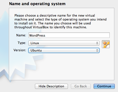
Step 3: open Virtualbox and hit the New button to create a new virtual machine. A window will open (see Figure 2) asking the name and OS for the new machine. Name it as you like, and choose Linux/Ubuntu as OS.
When asked for the amount of RAM, choose anything above or equal to 512MB. In the following window, choose "Do not add a virtual hard drive" and confirm your choice. After this step your new VM will be created, but you still have to explicitly link it to the disk image you previously created.
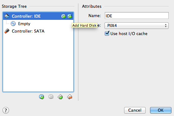
Step 4: choose your newly created VM and hit the Settings button. In the Storage tab you will find the list of disks attached to the VM (you should have only the "Empty" IDE CD if you followed the previous steps). Highlight Controller: IDE and click on the Add Hard Disk icon (see Figure 3). When asked whether to create a new disk or add an existing one choose the latter, then provide the path of the VDI image you created in Step 2.
Step 5: as a last configuration step, go to the Network tab and make sure your network adapter is enabled and configured as bridged (see Figure 4 - of course the adapter name might change according to which one is active in your system).
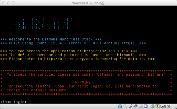
... Et voilà, the VM is ready: start it and if everything went fine you should be shown the following screen:
Note that you are provided an IP address (in this case 192.168.1.114): open your browser, connect to it and...
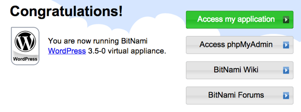
… enjoy! :-)
Octave clustering demo part 3: spectral clustering
[This post is part of the Octave clustering demo series]
This is (currently) the last of my posts devoted to clustering demos. If you haven't downloaded the file containing Octave code yet, you can get it here. If you want to read the previous articles, here they are: part 0 - part 1 - part 2.
The last demo in the package shows you how spectral clustering works. Spectral Clustering is a relatively recent approach to clustering that I found very interesting, especially because it addresses some of the limitations of k-means but, at the same time, it relies on k-means itself! What it does in practice is finding a new space where localities are preserved, emphasizing both the cohesion and the separation of clusters, thus allowing k-means to work at its best. If you are curious and want to delve deeper into this topic, you will find more material in the following page: Paper Review: A Tutorial on Spectral Clustering.
I was quite surprised not to find ready code for spectral clustering in Octave, but probably I just had not searched (well) enough. By the way, if you came here searching for it here is an(other?) implementation, together with some examples and data to play with: feel free to try it and to leave your feedback!
The spectralDemo function can be called as follows:
spectralDemo(dataset,nn,t)
where dataset is the usual dataset path+name, while nn and t are parameters used to build the (weighted) adjacency matrix describing similarity relationships between data points. Respectively, nn specifies the number of nearest neighbors for a point (a point is connected to another if it appears as one of its top nn nearest neighbors) and t is the parameter for the Gaussian similarity function s(xi,xj)=exp(-(xi-xj)^2 / t). My suggestion is to play with both parameters, but once you understood how they work you can just keep t=0 for the automatic tuning of the kernel and focus only on nn. Good values of nn range between 10 and 40, but of course you are free to test others (but keep in mind that the bigger the value, the slower the whole algorithm is! Can you say why?). The script performs the following tasks:
- it calculates the weighted adjacency matrix and plots both the distances between points and the weights between nodes in the adjacency graph (this allows one to inspect whether parameters need to be trimmed to have a more/less connected graph, and also to understand when the graph approach might work better than a classical euclidean distance approach);
- it builds the graph Laplacian and calculates its eigenvalues and eigenvectors. Then, it plots eigenvalues for inspection (this allows one to understand --if the dataset is clean enough-- how many connected components/natural clusters are present in the graph);
- to compare results between k-means and spectral clustering, it runs k-means both in the euclidean space and in the eigenspace built out of the top k eigenvectors, then shows both clusterings with related SSEs and accuracies.
And now, here are the usual maieutical questions:
- what are the datasets in which spectral clustering performs definitely better than k-means?
- how much do the results of spectral clustering depend on the input parameters?
- how would you evaluate the quality of a labeling done with spectral clustering? How would you apply that to find which is the best number of nearest neighbors to take into account?
- how often (according to your tests with different datasets) does the rule "the number of 0-valued eigenvalues matches the number of clusters" holds? How ofted does its "relaxed version" hold? (if the question is not clear check spectral clustering notes/papers)
- how worth would be to use algorithms other than k-means to do clustering in the eigenspace?
That's all... have fun with the demos and with spectral clustering :-)
